Using structural models

Determinism vs. statistics

Subsurface fracture problems are commonly attacked with statistical methods and several sections of this website (Part 8) are about fracture and orientation statistics. Section 1.3 is about deterministic prediction of the spatial location and intensity of fracturing. This discussion explains how these two very different approaches fit together.

An example of a statistical method.  Since 1990 a number of studies in many different geologic environments have shown that when fault size is plotted against fault density (surface area/unit volume) on a log-log plot, the result is a straight line, as shown in Figure 1. The slope and intercepts of the line vary, but the line is always straight. Saying that the fault population is "fractal" is just another way of saying the same thing.

Figure 1. Fractal fault-size distribution.

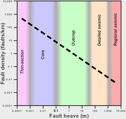
Joint populations appear to behave similarly and there are sound mechanical reasons for this relationship. The relationship appears to be constant from the scale of regional seismic surveys to the scale of individual grains within the rock. The beauty of this relationship is that because it is linear, the entire population can be characterized completely by observing it at any scale.

Statistics vs. Determinism.  The previous discussion leads to obvious questions like:

Why bother doing careful geology if I can know everything about the entire fault population all the way down to the grain scale just by counting faults in my seismic line/volume and calculating this groovy statistic?

To which there are two answers that depend on this key point:

If the data are apples, then a statistic is applesauce.

The answers are:

1. Whenever possible we want to know about the individual apples, not the sauce. Any statistic homogenizes heterogeneous data. Knowing the average fracture system of an entire field is useful because the small-scale character and variability can be modeled using Monte Carlo methods. However, we want to know where specifically the concentrations of fractures are and what the fractures there are like.
2. By calculating a statistic we state implicitly that we are making applesauce only with baskets of apples. If we accidentally add a basket of fish then the sauce is no good no matter how wonderful the fish are. When you present a statistic about a fracture population you implicitly state that the data came from a homogeneous volume. To calculate a useful statistic, you need to be sure that you are lumping data together from a homogeneously deformed volume and are not mixing data from two or more different volumes.

Devotees of fault-scaling methods will argue that answer #2 is incorrect because the population will have the same fractal dimension regardless of where you sample it. Even if they are right, answer #1 still holds. In other words, we don't want to know simply that there are heavily fractured areas out there somewhere, we want to know where they are, how big each one is, and how heavily fractured they are so that we can drill into, avoid, or correctly model them depending on our needs.

In short: It's a matter of scale.  The best approach for analyzing reservoirs is to use deterministic geologic methods to classify/specify the fracture character and distribution down to the smallest practical scale and then work stochastically at and below that scale. If time or data restrictions force us to work stochastically at an undesirably large scale we can still compute useful parameters, but the computed results and especially the final geological model(s) will not reflect reality as accurately as they would if the data were subdivided in a geologically meaningful way prior to statistical analysis and simulation.

Conclusion:  Deterministic geology should be used whenever practical to define reservoir volumes prior to statistical analysis.

When is a rock mass deformed enough to need quantitative structural analysis?

Section 1.3 is concerned with the general subject of using quantitative structural methods to define rock volumes that fractured during folding. If the rocks become fractured locally by folding then they must have started off as a homogeneously fractured or unfractured mass. Many oil fields, and many fractured reservoirs, occur in flat-lying, relatively undeformed rocks. How deformed do the rocks have to be before we need to treat them as heterogeneously fractured and use quantitative structural methods? To answer this question let's consider how a rock mass with a homogeneous fault population converts into a heterogeneous one by continued fault movement.

Figures 2 and 3 show some of the famous hoodoos at Bryce Canyon National Monument, Utah, U.S.A. The leading edge of a now inactive fold-thrust belt lies several miles to the left of the area shown in the photos. During propagation of the thrust belt, the rocks were deeply buried and were mechanically continuous with the fold-thrust belt. Erosion removed the overlying rock after the thrust belt became inactive. Bedding in the hoodoos is horizontal so it has not been disturbed by large-scale deformation. Two conjugate sets of small thrust faults with very little slip are readily visible. One set dips 30° to the left, one set dips 30° to the right, and the dip-azimuths of both sets are approximately perpendicular to the fold-thrust belt. The faults formed during propagation of the thrust belt and represent the earliest stage of failure of the strata. Even at this stage of development, slight fault-related folding of the strata is already evident on some of the larger faults. Had the fold-thrust belt continued to propagate, some of these faults would have grown and eventually would have produced folds like the ones described in Page 1.3.3.

Figure 2. Hoodoos at Bryce Canyon National Monument, Utah, U.S.A.

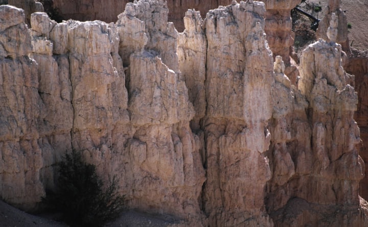
Notice that faults are present at all scales. The faults must be quite small because both terminations of many of them are visible and because many prominent faults do not visibly offset or fold bedding.

Figure 3. Detail of conjugate thrust faults in hoodoos at Bryce Canyon National Monument.

The planarity of the faults and the presence of two well-defined, contemporaneous groups suggests that the area shown in Figures 2 and 3 can be treated as a homogeneously deformed volume of rock. The fracture density should be fairly uniform because the fracture density was controlled by random nucleation of faults throughout the rock mass and the rocks are homogeneous, bedding is consistently horizontal and the rocks were probably stressed fairly uniformly because they are well forward of the leading edge of the fold-thrust belt. If this area was an oilfield then we would treat it as a statistically homogeneous volume.

Now let's imagine that the faults had continued to move so that fault-bend folds (Page 1.3.3) started to form. At what stage of fold development would we have to take localized deformation into account? Virtually any degree of fault-related folding is significant because the kink bands that are fault-bend folds can propagate indefinitely and even completely through the stratigraphic section and even a small increment of movement can form narrow, but extensive, fracture zones. Unfortunately, we can't use structural models to predict fractured areas if there isn't enough structural relief to detect in seismic data and we don't have other surface or subsurface structural data.

Conclusion.  Kinematic structural modeling should be used to define structural domains whenever detectable fault-related fold structures can be resolved with available data.

Bulk strain does not predict fracture type or density

The pages in section 1.3 show how quantitative structural models are used to predict the bulk rock strain caused by various types of folding from accurate representations of subsurface structure. Since modern seismic data is an excellent source of subsurface structural information, it should be possible to develop a relationship between strain and fracture density (fracture surface area/unit volume) or other fracture system properties, as shown in Figure 4. With such relationships, we should be able to predict fracture system properties in advance of drilling and use this information to optimize exploration and development wells and to build accurate geologic and engineering models of a reservoir. Unfortunately, we need more information than just the bulk strain to accomplish these goals.

Figure 4. Strain vs. fracture density.

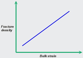
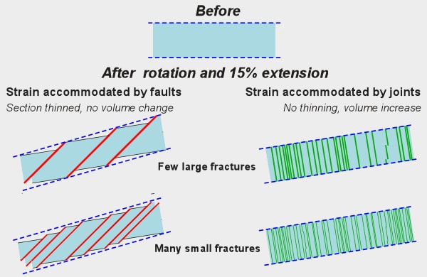
Relationships between strain and fracture properties must be developed and calibrated for an area of interest using subseismic-scale data because strain predictions from structural models are useful for predicting the spatial location of fracturing, but say nothing about important fracture system properties such as the number, type, orientation, density, size distribution, permeability, porosity and stratigraphic heave distribution (in the case of faults) of each fracture set. Bulk strain information alone cannot predict fracture properties because a given bulk strain can be accommodated by fracturing in an infinite number of ways. Figure 5 shows how a fixed amount of extension of a single bed can be accomplished by different densities of either joints or faults.

Figure 5. A fixed amount of extension can be accommodated by joints or faults in an infinite number of combinations.

Conclusion:  Bulk strain alone is not a predictor of fracture system properties.

Predicting fracture type from first principals

Joints or faults? It matters.  Different fracture types form in different orientations relative to the principal stresses, have different termination relationships, fluid-flow behavior, relationships to other types of fractures and geologic structures, and size/shape distributions. A method of predicting fracture type without subseismic-scale data would clearly be useful. We know that knowledge of the bulk strain alone is insufficient to determine fracture type, but perhaps bulk strain data combined with other information would be sufficient to theoretically predict fracture type. We'll discuss fracture-type prediction in terms of joints vs. faults because these are the two most common fracture types and have very different fluid-flow properties.

The left and right sides of Figure 5 clearly would exhibit different fluid-flow behavior. Note that idealized, planar faults accommodate strain without producing any porosity or permeability but joints increase the porosity and permeability of the rock mass. In nature faults can be barriers to fluid flow, can be highly permeable or anything in-between.

Figure 6: Fracture type and lithology.  Individual lithologies often fracture differently, and even interbedded lithologies with different mechanical properties may develop different types of fractures as illustrated in Figure 6. When interbedded lithologies develop different types of fractures, the amount of strain is equal in each lithology. Note that permeable joints may provide no communication perpendicular to bedding if they are only developed in one lithology in an interbedded sequence of two or more lithologies.

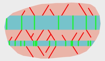
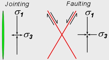
Figure 7: Joints or faults?  The type of fractures that form in a rock are a function of the mechanical properties of rock (such as strength) and the effective stresses in the rock during deformation. Joints form when the minimum principal effective stress is tensile. Faults form when all of the effective stresses are compressive and there is a sufficiently large difference between the maximum and minimum principal stresses. Figure 7 shows the relative magnitudes of the stresses during jointing and faulting.

Stress state.  The stress state of a rock mass is described by the orientations and magnitudes of all three principal effective stresses. The effective stress state is a function of three factors:

• The internal properties of the rock mass, which are the pore pressure and the rock's mechanical properties such as the elastic moduli and Biot's constant.
• The applied stresses, which we will define as stresses resulting from movements of the boundaries of the rock mass by external forces.
• The pore pressure.

Sources of applied stress.  It's convenient to think of two sources of applied stress when we think about how fractures develop during folding:

• The regional stresses (also called the remote or far-field stresses).
• Stresses resulting from strains (distortions of the rock mass) required to accommodate folding.

Can we predict fracture type from first principals?  If we know the rock mechanical properties, layer thicknesses, pore pressure and remote stresses at the time of fracturing and we know the strains required by folding, then in theory we should be able to predict the fractures that developed. In practice, this information can be hard or impossible to know with confidence, although often reasonable estimates can be made. Several groups are working on this issue and some software packages are available for mechanically modeling fracture growth. However, the answer to the question is: No. In general fracture type and other fracture system properties cannot be predicted confidently from first principals.

However, knowledge of the strains produced by folding can accurately predict the spatial location of fracturing and can help estimate the orientations of fractures.

OK. So how do we develop an accurate understanding of subsurface fracture systems?  We do this by:

• Using subseismic scale data to develop statistical characterizations of the fracture system within structural compartments as defined by quantitative structural analysis.
• If we don't have subseismic data (core, image logs etc.) then we attempt to determine the fracture system properties by downscaling seismic-scale data.
• Characterizations are then extrapolated throughout the volume of their compartments. We can improve or supplement this approach with forward modeling. (Forward mechanical models attempt to reproduce the observed subsurface fracture system from first principals by mechanically modeling deformation and growing the fracture system.)

Practical application of these methods

Wildcat drilling.  Wildcats should be drilled in structural domains that are expected to be more heavily fractured, such as such as shown on page 1.3.3, for example domain F3 in Figure 6 or the transversely extended domain shown in Figures 8 and 9.

Exploration and delineation drilling.  Exploration and delineation drilling should attempt to sample each structural domain prior to development drilling.

Reservoir characterization.  Structural localization of fracturing has two critical implications for fractured reservoir characterization:

• Data from different structural domains should not be combined when making bulk characterizations. For example: Data on fracture orientation and location within a wellbore are used to generate discrete statistical models of subsurface fracture networks. Well data from different domains MUST NOT be combined prior to statistical analysis because the properties of each domain may be different.
• At least one complete suite of reservoir data should be collected in each structural domain. Utilizing this data-collection methodology can reduce logging costs by optimizing the types and amounts of data acquired in each well. I emphasize that cost-effective may or may not equal cheap. Cost savings are realized by ensuring that each structural domain is characterized with the minimum number of wells. Always remember: Correct reservoir simulation depends on sound reservoir characterization, which is impossible without adequate data. Most essential fracture characterization data are collected in open holes. Skimping on logging and testing programs when a well is drilled can save a small amount of money up front. However, not collecting adequate data sets during drilling can cost vastly larger sums later in the life of the field when attempting to deal with problems such as premature water breakthrough, bypassed oil, pressure maintenance, and secondary recovery. In one famous fractured reservoir (that shall remain nameless) the company skimped on the logging program to save money during development. Years later the lack of data directly resulted in the loss of as much as 200 million barrels of oil. Although the amount of unrecovered oil in this field will never be known accurately, collecting a good data set and doing a first-class workup clearly would have been orders of magnitude more cost-effective.

Note that a single well can sample more than one structural domain if the well trajectory is planned correctly. Read the section on "Recommendations for drilling and logging fractured reservoirs" for discussion of data collection methods and well planning.

Reservoir simulation.  Numerical reservoir simulators use three-dimensional models of subsurface fluid-flow and fluid-storage properties to calculate reserves, reservoir performance, plan development and enhanced-recovery strategies, and other critical tasks. Fractured reservoir simulators must incorporate the effects of fractures on rock mass fluid-flow properties, which presents a problem: Subsurface fracture networks are characterized primarily from wellbore data, but wellbores provide only tiny samples of the reservoir. Structural models of the reservoir provide a way to extrapolate wellbore data throughout the reservoir volume. Fracture characterizations should be extrapolated throughout and only within the structural domain that was the source of data for the characterization.

Structural models and seismic data.  Seismic velocities and anisotropy are often used as indicators of fracture properties. Unfortunately, seismic data alone are not adequate to characterize reservoir fracturing because fracture systems have many more variables than the complete seismic velocity tensor. However, seismic data are extremely valuable when used to leverage, test/corroborate, or extend other data sets. In the context of quantitative structural models, seismic information has the potential to delineate fracture domains directly and may indicate the relative intensity of fracturing in each structural domain. The limitation is that fracture properties such as the number, density (surface area/unit volume), size distribution, and fracture-derived permeability cannot be predicted from seismic data.